Enhancing green hydrogen forecasting with a spatio-temporal graph convolutional network optimized by the Ninja algorithm

To make the modeling of the hydrogen data systematic and reproducible, an end-to-end pipeline was created and is summarized graphically in Fig. 1. Joining together a set of key steps, namely raw data preprocessing to the final model evaluation, the workflow exploits classic and contemporary optimization procedures. To perform the procedure, one must first obtain a dataset that includes the environmental and operational parameters of hydrogen systems. The raw data is then subjected to a significant data preprocessing phase, during which vital quality aspects are detected and handled. The step will consist of processing steps like missing value processing, normalization, feature scaling, outlier processing, and categorical encoding. These transformations are necessary to ensure the data is ready for robust and unbiased learning.

Comprehensive pipeline for hydrogen data modeling, incorporating data preprocessing, dataset splitting, metaheuristic-based feature selection, model training with baseline architectures, and final performance evaluation.

After preprocessing is complete, the data is divided into training and testing sets in an 80:20 ratio. Model development and hyperparameter tuning are performed on the training data, and the testing data is kept aside until the final evaluation to avoid biased performance estimation. To efficiently learn and reduce dimensionality, the feature selection stage is essential. It is carried out using a variety of metaheuristic optimization algorithms, namely bNinja, bFA, bTSH, bPSO, bJAYA, bFEP, bGSA, bQIO, bWOA, and bAPO. All these algorithms are coordinated by the central Ninja Optimizer module that acts as an intelligent search through the search space to find the most informative feature subsets. After feature selection, a set of baseline models, consisting of STGCN, DTCN, TCN, DKLT, LSTM, CTSM, and FTLM, is fitted on the low-dimensional feature space. The models represent a range of different deep learning architectures and temporal learning paradigms, enabling highly competitive benchmarking. Finally, the performance evaluation block will compute several performance measures used to assess the predictive accuracy and generalizability of each model. The reason this is done is to validate the whole working process quantitatively, from data ingestion to prediction.

Dataset description

This work is based on the Renewable Hydrogen Production Dataset, a multidimensional and comprehensive dataset of environmental, technological, and geographical variables spanning 2535 cities worldwide. The dataset is explicitly tailored to this end, modeling and analyzing the potential for producing green hydrogen across a wide variety of urban and regional geographies, with a strong emphasis on sustainability and environmental applicability. It has been selected, based on its scope and scientific usefulness, to provide an empirical basis for the development of intelligent and resource-conscious hydrogen infrastructure in international decarbonization plans. In the dataset, each data record comprises crucial indicators of renewable energy potential, such as solar irradiance and wind speed, as well as extensive system characteristics, including photovoltaic (PV) and wind power generation, electrolyzer efficiency, and overall system efficiency. Such a combination of features facilitates fine-grained spatial modeling, making the dataset particularly interesting to those seeking to understand where green hydrogen is most promising to deploy. The resource-rich and coastal areas will gain enormously, as even the desalination power demand has been factored in to enable a realistic assessment of water resource limitation in hydrogen electrolysis. Moreover, because the dataset includes environmental factors and operational indicators in equal measure, the data become useful in integrative analyses used to guide ecological planning, investment priorities, and policy-making. To enhance clarity and guided analysis, the essential characteristics of the dataset are summarized in Table 2, with each feature defined by its functional usefulness in predicting hydrogen production. Remarkably, environmental conditions, which include solar irradiance (in kWh/m²/day), wind speed (in m/s), and ambient temperature (in °C), are necessary for calculating the renewable energy yield and the system efficiency. In the meantime, such technological characteristics as the PV and wind power generation (in kW), desalination power demand (in kW), and electrolyzer efficiency (in %) provide an idea of the engineering performance of a hydrogen production process. The geospatial identifiers (Latitude, longitude, etc.) support these variables and allow spatial interpolation and regional optimization modeling. The combination of the mentioned dimensions makes the dataset a key resource for modeling hydrogen production based on environmental foundations. To facilitate the intensive machine learning analysis, the dataset is divided into two disjoint subsets: a training set to fit the model parameters and extract patterns, and a test set to assess the model’s generalization performance solely. This layered separation yields predictive results that are statistically sound and environmentally explainable, reducing overfitting and algorithm bias in empirical assessments.

Renewable energy sources Analysis involves a deep insight into the input parameters involved. Figure 2 shows important distributions of solar energy and wind energy. The distributions of several subplots in Fig. 2 are displayed as kWh/m²/day. Hence, the first subplot demonstrates the distribution of daily solar irradiance, which is roughly symmetric and seems to be concentrated around 4-6 kWh/m²/day, which means that solar exposure is consistent throughout the dataset. The distribution of the speed of wind (in m/s) is presented in the second subplot in Fig. 2. This occurrence is skewed to the right, implying that lower wind speeds may be more frequent and there is a lower incidence of high wind speeds. The third subplot of Fig. 2 shows the distribution of the photovoltaic (PV) power generation (in kW). As may be expected, it closely tracks the solar irradiance pattern since the two variables are directly related. Figure 2 shows the renewable power distributions, where the fourth subplot is the wind power output (in kW), which is heavily skewed to the right. This shows that low wind power output is observed most of the time, and high power output is comparatively infrequent. Finally, the fifth subplot in Fig. 2 displays the distribution of the aggregate renewable energy, which includes both wind and PV power. It resembles the distorted shape of wind power distribution, indicating a high contribution of wind power and its associated variability to overall renewable energy generation.

Distributions of key renewable energy variables: Solar irradiance, wind speed, PV power, wind power, and total renewable energy.

The characterization of hydrogen production variability in geographically diverse climatic and operational conditions is crucial for optimizing renewable energy strategies. The comparative distribution of hydrogen production under the influence of different factors is in Fig. 3. The factors of hydrogen production by Fig. 3 show the first subplot of hydrogen production by Latitude Band. Equatorial and temperate regions tend to have higher median production, whereas subtropical and tropical regions have comparatively low outputs. There is a high variability in the polar band, which is probably caused by the drastic seasonal fluctuations. In the second subplot of Fig. 3, hydrogen production is clustered by Seasonal Variation. The greater seasonal variation appears to correlate with the higher variability and maxima of hydrogen production, suggesting that seasonality may contribute significantly to production efficiency. The third subplot of Fig. 3 considers the Seasonality Type to analyze hydrogen production. Both polar and seasonal regions are broader, with higher medians, than the tropical regions, which are more stable but have lower hydrogen production. Lastly, in Fig. 3, the fourth subplot considers the Efficiency Class of the systems. Although there is overlap in the range of all the efficiency classes, systems with higher efficiency have a slightly higher median and lower variance in hydrogen production, which means that their performance is more predictable.

Boxplots showing hydrogen production (kg/day) as influenced by latitude band, seasonal variation, seasonality type, and efficiency class.

Data preprocessing

Preprocessing is one of the essential steps in preparing raw data for use in further modeling, especially in the case of deep learning-based environmental forecasting³⁵. The scale of the renewable hydrogen production dataset, which features a wide range of continuous and potentially correlated environmental and operational variables, will necessitate a systematic and stepwise preprocessing pipeline designed to enhance data quality, remove noise, and make the data amenable to interpretation by a model. The first step of this pipeline is data cleaning and imputation. Actual environmental data often fail to comply with gaps or inconsistencies in the recordings due to sensor malfunctions, data recording errors, or the inherent variability in the measurement rate. To address missing values, statistical imputation techniques are employed. In particular, for numerical attributes (e.g., ambient temperature, solar irradiance, and renewable power outputs), missing values are imputed using central tendency estimators (most typically the mean or median) selected according to the underlying distribution and the presence of outliers. In cases of categorical features, they will be encoded using One-Hot Encoding (OHE), thereby converting nominal variables into a binary representation without imposing an ordinal structure on the data that could generate spurious model behavior. After imputation, feature engineering and correlation analysis steps are performed to enhance the signal-to-noise ratio in the data. Strongly correlated (or redundant) features can obscure any actual causal structure and lead to multicollinearity, which can make model learning unstable, especially in neural models where the features are assumed to be independent. The features are checked to see if they have a linear dependency by calculating a Pearson correlation matrix. The variables with correlation coefficients higher than a specified value (usually \(r > 0.9\)) are removed, or a transformation is done. This procedure helps retain only the most informative features, which are not duplicated, resulting in more interpretable and simpler models. After the dimensional refinement, feature scaling is done to standardize the scale of all the continuous attributes. Since the units are diverse, for example, irradiance can be expressed in kilowatt-hours per square meter per day and hydrogen production in kilograms per day, the raw feature values can vary by different orders of magnitude. To reconcile such differences, the variables are Min-Max normalized to reshape them to a standard range, typically [0, 1]. It is essential in gradient-based learning algorithms, where the scales of different features are disproportionate, as this can cause unstable convergence or biased learning paths. Further standardization may be necessary in some instances to meet the requirements of models with specific input parameters. As another example, recurrent neural networks (RNNs), such as Long Short-Term Memory (LSTM) networks and transformer-based models, like the Deep Kernel Learning Transformer (DKLT), are sensitive to the properties of input distributions. In these models, optional z-score standardization is sometimes used, transforming features into a standardized form with a mean of zero and a variance of one. Such transformation is determined conditionally and is specific to the empirical performance of each deep learning architecture during its early testing stages. Together, these preprocessing plans – encompassing imputation, encoding, scaling, and standardization – are designed to create a meaningful and analytically straightforward dataset. This enables the consistent training of deep learning models for predicting environmentally relevant hydrogen production, ensuring that model outputs are both statistically and environmentally meaningful. Preprocessing is one of the essential steps in preparing raw data for use in further modeling, especially in the case of deep learning-based environmental forecasting³⁵. The scale of the renewable hydrogen production dataset, which features a wide range of continuous and potentially correlated environmental and operational variables, will necessitate a systematic and stepwise preprocessing pipeline designed to enhance data quality, remove noise, and make the data amenable to interpretation by a model. The first step of this pipeline is data cleaning and imputation. Actual environmental data often fail to comply with gaps or inconsistencies in the recordings due to sensor malfunctions, data recording errors, or the inherent variability in the measurement rate. To address missing values, statistical imputation techniques are employed. In particular, for numerical attributes (e.g., ambient temperature, solar irradiance, and renewable power outputs), missing values are imputed using central tendency estimators (most typically the mean or median) selected according to the underlying distribution and the presence of outliers. In cases of categorical features, they will be encoded using One-Hot Encoding (OHE), thereby converting nominal variables into a binary representation without imposing an ordinal structure on the data that could generate spurious model behavior. After imputation, feature engineering and correlation analysis steps are performed to enhance the signal-to-noise ratio in the data. Strongly correlated (or redundant) features can obscure any actual causal structure and lead to multicollinearity, which can make model learning unstable, especially in neural models where the features are assumed to be independent. The features are checked to determine whether they have a linear dependency by calculating a Pearson correlation matrix. The variables with correlation coefficients higher than a specified value (usually \(r > 0.9\)) are removed, or a transformation is done. This procedure helps retain only the most informative features, which are not duplicated and which contribute to interpretability and simpler models. After the dimensional refinement, feature scaling is done to standardize the scale of all the continuous attributes. Since the units are diverse, for example, irradiance can be expressed in kilowatt-hours per square meter per day and hydrogen production in kilograms per day, the raw feature values can vary by different orders of magnitude. To reconcile such differences, the variables are Min-Max normalized to reshape them to a standard range, typically [0, 1]. It is essential in gradient-based learning algorithms, where the scales of different features are disproportionate; this may cause unstable convergence or biased learning paths. Further standardization may be necessary in some instances to meet the requirements of models with specific input parameters. As another example, recurrent neural networks (RNNs), such as Long Short-Term Memory (LSTM) networks and transformer-based models, like the Deep Kernel Learning Transformer (DKLT), are sensitive to the properties of input distributions. In these models, optional z-score standardization is sometimes used, transforming features into a standardized form with a mean of zero and a variance of one. Such transformation is determined conditionally and is specific to the empirical performance of each deep learning architecture during its early testing stages. Together, these preprocessing plans – encompassing imputation, encoding, scaling, and standardization – are designed to create a meaningful and analytically straightforward dataset. This enables the consistent training of deep learning models for predicting environmentally relevant hydrogen production, ensuring that model outputs are both statistically and environmentally meaningful.

Deep learning models

This study employs a diverse range of deep learning models, each with its distinct capabilities to learn from high-dimensional, sequential, and geospatially structured data, to identify the most effective model for representing the complex temporal and spatial patterns underlying green hydrogen production. Such models are especially suited to applications in environmental science, where accurate prediction requires not only the recognition of the dynamism of renewable energy resources but also the consideration of contextual effects from geographic and system-level factors.

The Spatio-Temporal Graph Convolutional Network (STGCN) serves as one of the core elements of the modeling framework, as it has the potential to preserve both spatial correlations and temporal dependencies. STGCN learns the topology-based correlation among cities based on geographic and infrastructural similarity using graph convolutional layers. At the same time, gated temporal convolutional encoding enables it to capture sequential behaviors in hydrogen production due to diurnal patterns, seasonality, and variability in weather patterns. This architecture is instrumental in situations where the geometrical organization of data is a crucial factor, as is the case with decentralized hydrogen networks connecting multiple cities.

The other architecture used is the Dynamic Temporal Convolutional Network (DTCN) that improves temporal feature extraction with dynamic convolutional receptive fields. Such flexibility is essential for learning non-stationary time series, such as those observed in solar and wind energy inputs, where variability in both time and amplitude is typical.

The Temporal Convolutional Network (TCN) is also added because it is efficient in handling long-range temporal dependencies. Through the use of dilated convolutions and residual connections, TCN can learn long temporal patterns and, by doing so, emphasizes the benefits of avoiding the vanishing gradient problem typically seen with recurrent models.

The Deep Kernel Learning for Time Series (DKLT) model integrates deep neural representations with kernel-based methods (e.g., Gaussian Processes) by incorporating probabilistic reasoning. This hybrid scheme not only allows for deterministic prediction but also accommodates the quantity of uncertainty, a mandatory attribute in environmental forecasting when incomplete or noisy data is present.

A Recurrent Long Short-Term Memory (LSTM) network is applied due to its efficiency in modeling long-term temporal sequences. It features gated recurrent units that can effectively capture longstanding environmental rhythms, which explains why it aligns well with energy generation and hydrogen production data that tend to exhibit seasonal and periodic trends.

Along with this, the Continuous-Time Sequence Model (CTSM) presents a time-based modeling structure that supports unequally spaced data points, which are typical in realistic settings of environmental monitoring. CTSM offers a mathematically precise approach to model asynchronous data acquisition with no artifacts of temporal discretization.

The Federated Temporal Learning Model (FTLM) enables training a distributed model across multiple data silos, which is especially important in cases where data sovereignty and regional data protection are paramount. FTLM is also consistent with the new tenets of sustainable and ethical data science, providing a distributed strategy for learning models and ensuring the integrity of local data. The STGCN model has been identified as the most promising architecture among those targeting hyperparameter optimization. Its ability to learn both spatial and temporal dependencies jointly leads to its steady good performance at the baseline, which naturally presents a straightforward target for improvement. By utilizing enhanced optimization methodologies that incorporate metaheuristic search procedures, this model is optimized to achieve higher predictive and computational performance, thereby yielding more stable and high-performance forecasting of renewable hydrogen production in environmentally dynamic situations.

Metaheuristic algorithms

Optimization is a key aspect in the context of environmental modeling (especially in high-dimensional, data-driven applications, such as green hydrogen production forecasting) to improve accuracy and computational efficiency. Common approaches often struggle to deal with nonlinearities, heterogeneities, and the scale of such data. Metaheuristic algorithms are an attractive alternative, inspired by natural and physical phenomena, to carry out robust and adaptive searches on complex landscapes. Their random, though clever design enables them to efficiently manage tasks such as feature selection and hyperparameter tuning, which are essential to maximizing the performance of deep learning. This section discusses the strategic role of metaheuristics within the proposed modeling scheme, explaining their contributions to dimensionality reduction and parameter optimization. It also presents the new Ninja Optimization Algorithm (NiOA), a biologically inspired and exploration-exploitation balanced optimizer. It compares its performance to a collection of well-known benchmark algorithms in both binary and continuous search spaces.

Role in feature selection

The dimensionality reduction approach employed in this paper utilizes metaheuristic algorithms as a core element. Since a vast number of input variables are generated based on environmental, technical, and geographical factors, the feature space related to renewable hydrogen production forecasting is high-dimensional and perhaps redundant. Conventional deterministic algorithms can be inadequate for searching such a high-dimensional space, especially when the objective function is non-convex or contains numerous local optima. To the contrary, metaheuristics offer a random (stochastic) but informed mechanism of global search and optimization. Metaheuristic algorithms iteratively search the feature space, attempting to select the most informative subset of variables by analogy with natural processes, such as biological evolution, swarm behavior, or physical phenomena. The procedure enables the model to retain features with the most predictive relevance and discard features that introduce noise, redundancy, or computational overhead. By promoting the better generalization capacity of deep learning models, feature selection also has the beneficial effect of dramatically decreasing both training time and energy requirements, which are of paramount importance in sustainable computational modeling. Also, the dimension of the selected feature subset can be considered an advantage because it leads to better interpretability, especially meaningful in an environmental context where a clear indication of the contribution of variables is policy and planning-relevant.

Role in hyperparameter optimization

Besides using them in feature selection, metaheuristic algorithms are also employed for hyperparameter optimization. Particularly, deep learning models, such as those with intricate structures like the Spatio-Temporal Graph Convolutional Network (STGCN), are susceptible to hyperparameters, including but not limited to the learning rate, the number of layers, filter size, batch size, and dropout rate. These hyperparameters can be tuned manually, but the process can be laborious, time-consuming, and prone to failure in finding optimal settings, as the parameter space is high-dimensional and dependent. Metaheuristic optimization automates this procedure by searching the hyperparameter space adaptively with population-based methods. These algorithms evaluate the performance of models across various parameter settings and converge on those that yield better predictive accuracy and stability. Hyperparameter optimization in the case of the STGCN model is particularly highlighted in this study, as this model yielded the best results on the baseline. The model can be optimized concerning its architecture and training parameters using metaheuristic techniques, thereby yielding a significant improvement in its ability to generalize in spatially heterogeneous areas. Such an automated workflow not only speeds up the model development pipeline but also makes the deployment of computing resources more robust and environmentally friendly.

Proposed optimizer: Ninja optimization algorithm (Ninja)

In this paper, we introduce the Ninja Optimization Algorithm (NiOA) as a state-of-the-art and context-aware metaheuristic framework that can be applied to two tasks of primary significance in deep learning pipelines: feature selection and hyperparameter optimization. NiOA is specifically designed to navigate the complexity of high-dimensional and multi-modal search spaces, which are typical of environmental prediction problems, such as spatiotemporal modeling of renewable hydrogen production. Inspired and informed by the nimbleness, sneakiness, accuracy, and motion adaptation techniques of ancient Japanese ninjas, NiOA incorporates these behavioral themes into a mathematically grounded Optimization framework that effectively performs both global and local searches. In its most basic form, NiOA is structured to have two fundamental behavioral stages, exploration and exploitation, which work together to offer the trade-off between global search and local refinement. During the exploration phase, agents (named in this case ninjas) are passed dynamically and oscillatory through the solution space to escape local optima and to promote diversity. The position is updated, Exploration as:

with \(Ls(t)\), \(Ds(t)\) being two interacting solution vectors, \(r_1\), \(r_2\) adaptive random coefficients and \(FS\) the feasible solution space. Cosine-based perturbations introduce periodic, controlled variability that enhances the optimizer’s ability to escape local minima and reduce variance, allowing it to explore global regions more effectively. In further diversification of the search, NiOA includes a mutation mechanism, which carries out perturbation according to a nonlinear series:

where \(a \in [6,10]\) is an randomly chosen integer, and \(x\) is the current solution. The non-uniform, alternating updates in this equation aim to emulate stealth-like, jagged movements, making the search less prone to premature convergence, a key shortcoming of classical algorithms, such as Genetic Algorithms (GA) or Particle Swarm Optimization (PSO). During the exploitation phase, NiOA increases the search intensification in and around high-fitness areas with gradient-free adaptive heuristics. Solution refinement is modeled by:

where \(J_1, J_2\in [0,2]\) are constants of tuning that control the rate of convergence and accuracy. This formulation can be leveraged in a memory-aware manner with adaptive step control, which dynamically adjusts the search intensity based on the curvature of the fitness landscape. Further polish is brought in by:

This introduces nonlinearity in the exploitation dynamics, allowing for finer-grained control over convergence trajectories and escape strategies as needed. When no progress has been noticed after a certain number of iterations, NiOA triggers a stagnation-handling mechanism to re-diversify the population:

where the stochastic control parameters are \(i, n, v_s \in [0,2]\). Without completely resetting the solution state, this technique successfully reintroduces Exploration into the optimization pipeline by using composite-directed updates. NiOA can be applied in feature selection based on NiOA in binary form (bNiOA) using sigmoid transfer functions to map the continuous positions of the agents to binary quantities (0 or 1), which is an indicator that a feature is excluded (0) or included (1). The adaptation enables NiOA to select small yet highly informative feature subsets, which alleviates overfitting, makes models more interpretable, and scales up to large computations. Experimental findings from benchmark experiments reveal that bNiOA uniformly outperforms classification errors, the number of selected features, and the variation of fitness scores compared to standard binary optimizers, bTSH, bFHO, and bSAO. Within the scope of hyperparameter optimization, the fact that NiOA can optimize the learning rate, dropout rate and the number of filters/layers is used to improve the generalization of deep learning models. This is particularly true for spatiotemporal models, such as STGCN, where the complexity of the data differs in both the spatial and temporal domains. Compared to the classroom, NiOA has demonstrated improved convergence behavior and generalization strength over more traditional trial-and-error-based methods, gradient-based optimization methods, and grid/random search-based methods. In total, the rich mathematical formulation of NiOA, which encompasses dynamic exploration-exploitation control, nonlinear learning strategies, and biological adaptation analogies, makes a significant contribution to the domain of metaheuristic optimization. Its embodiment into a renewable hydrogen forecasting system does not just offer concrete benefits in the form of model performance gains. Still, it also corresponds to the computational and ecological urgency of environmental science modeling, offering optimization with both rigor and efficiency.

Algorithmic framework of the Ninja optimizer

Algorithm 1 formally summarizes the computational behavior of the Ninja Optimization Algorithm (NiOA), which is described in detail in the following: The evolutionary process that is used to address optimization problems in two different paradigms: (i) feature selection with the binary adaptation of NiOA (bNiOA), and (ii) hyperparameter tuning of deep learning models, where NiOA is deployed in its continuous variant. In the feature selection task, the NiOA algorithm is adapted into a binary search version (bNiOA). Still, here, the decision vector indicator of whether to include or exclude input features is passed through a sigmoid transfer function. In the given case, a ninja agent is a binary string encoding a subset of features that have been chosen. The task is to minimize the risk of classification error as much as possible while also reducing dimensionality, thereby enhancing model generalization and training speed. The exploration, mutation, and exploitation stages are iterated during the optimization process to successively improve the binary solutions, preferring sparse but informative feature subsets. When used in the context of hyperparameter optimization, NiOA is used in its continuous real-valued deployment. The solution vector code represents a configuration of tunable parameters, including the learning rate, dropout probabilities, hidden unit count, convolution kernel sizes, or temporal window lengths, depending on the specific deep learning architecture being optimized. The optimizer is a procedure that varies these parameters to minimize an error-based cost function (e.g., validation loss or prediction error) and can dynamically explore the parameter space through position updates, nonlinear perturbations, and adaptive learning heuristics. The same basic algorithmic framework is used in both forms of NiOA: binary NiOA (feature selection) and continuous NiOA (hyperparameter optimization). That algorithm is given in Algorithm 1. This framework comprises agent position initialization, an alternating mechanism between exploration and exploitation, a stochastic mutation operation, and an update mechanism to handle stagnation and escape local optima. Continuous and binary encodings differ solely in the way the search space and candidate solutions are represented and defined.

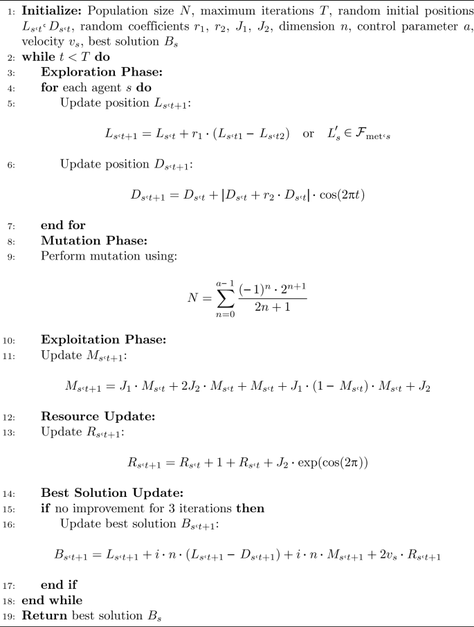
Ninja Optimization Algorithm (NiOA)

The NiOA framework’s flexibility and generalization enable it to smooth interchange between binary and continuous search spaces, thereby offering a unified optimization engine for a wide variety of tasks in deep learning pipelines. That renders NiOA especially beneficial in environmental modeling applications with both high model dimension and nonstationary high-dimensional data.

Benchmark optimizers for comparison

To thoroughly test the strength, precision, and computational performance of the proposed Ninja Optimization Algorithm (NiOA), we compared its performance with a selected set of modern metaheuristic optimizers. These algorithms traverse a spectrum of bio-inspired and physics-based paradigms and have been widely popular in the optimization literature for their effectiveness in tackling complex, high-dimensional, and multimodal problems. The comparative analysis of feature selection and hyperparameter optimization tasks provides a comprehensive evaluation of NiOA in terms of adaptability and generalization to different optimization spaces. The standard algorithms are:

• FA – Firefly Algorithm In FA, attracted by the bioluminescent communication of fireflies, the swarm intelligence algorithm was proposed, where the brightness-based attraction modeling provides the global and local search capacities.

• TSH – Tunicate Swarm Hybrid Optimizer A hybrid algorithm based on the feeding behavior of tunicate, which has cooperative foraging behaviors. Although it is comparatively new, TSH has confirmed a competitive convergence rate and solution diversity.

• PSO – Particle Swarm Optimization A well-known and old algorithm inspired by the collective motion of bird flocks and fish schools. Every agent changes its velocity and position according to the personal and social best positions.

• JAYA – Success-Based Optimization JAYA is a parameter-free algorithm that iteratively pushes the population towards the optimal solution and away from the worst solution, making it computationally appealing due to its simplicity and efficiency.

• FEP – Fast Evolutionary Programming An adaptation of the classical evolutionary programming to ensure better convergence and less computational baggage via effective mutation schemes.

• GSA – Gravitational Search Algorithm A physics-based algorithm based on the simulation of mass interactions under Newtonian gravity, where the agents with greater mass attract the lighter agents, resulting in exploration based on fitness.

• QIO – Quantum-Inspired Optimization Using the concepts of quantum mechanics, including superposition and entanglement, QIO enables a probabilistic search procedure that allows for a broad-area search during the initial stages and subsequently narrows down the search space.

• WOA – Whale Optimization Algorithm WOA employs spiral-shaped movement patterns to dynamically switch between exploration and exploitation, modeled after the bubble-net hunting method of humpback whales.

• APO – Anomalous Particle Optimizer One recently introduced algorithm that combines statistical anomaly detection with swarm behaviors to focus exploration on solution regions that are rarely sampled.

All the algorithms were thoroughly investigated in the same experimental conditions: the same datasets were used, as well as the same evaluation measures, population sizes, and stopping criteria. The latter comparative framework provides methodological consistency, enabling the objective and reproducible assessment of NiOA’s performance in both discrete (binary) and continuous search spaces.

Evaluation metrics

To guarantee the multidimensionality of the assessment of performance, two types of evaluation measures were used: forecast metrics to assess the quality of model predictions and feature selection metrics to assess the quality of dimensionality reduction.

Forecast evaluation metrics

Forecast evaluation metrics are measures of the accuracy, bias, variability, and explanatory power of model predictions. They are essential in environmental forecasting models, where precise numerical prediction of hydrogen production, system efficiency, or energy use is required. These metrics provide a standardized way to assess how well a model captures observed patterns and whether it tends to systematically over- or under-predict outcomes. For instance, error-based metrics, such as the Mean Squared Error (MSE) and Mean Absolute Error (MAE), quantify the deviation between observed and predicted values, while correlation-based measures, such as the coefficient of determination (\(R^2\)), evaluate the explanatory power. A summary of commonly used evaluation metrics and their mathematical formulations is presented in Table 3.

Feature selection evaluation metrics

The performance of feature selection is evaluated by the degree to which the selected subset of features reduces the dimensionality of the input data while preserving or enhancing the predictive accuracy of the model. This is particularly important in environmental applications, where the input variables (such as climate parameters, energy measures, and geographic attributes) are often high-dimensional, leading to challenges such as multicollinearity, noisy patterns, and potential overfitting. Evaluation metrics are therefore necessary to quantify both the quality of the selected features and the consistency of the selection process across multiple runs. Table 4 summarizes the most common metrics used for assessing feature selection performance and their corresponding mathematical formulations.

All these metrics together enable a fine-grained analysis of how each optimizer performs under different conditions, allowing for statistical comparison (e.g., ANOVA, Wilcoxon tests). Capturing predictive, structural, and computational aspects of model quality jointly ensures that the identified optimization strategies are not only practical but also scalable and interpretable in environmental science applications.