Economic and environmental competitiveness of multiple hydrogen production pathways in China

Overview of hydrogen production pathways

Each hydrogen production pathway needs to achieve the same hydrogen supply reliability (hydrogen supply rate) for a fair comparison of LCOH. More than 90% of the global hydrogen used in industrial applications such as refining, ammonia synthesis, and methanol preparation, a stable supply of hydrogen is an absolute requirement for safe industrial production¹². Most hydrogen production equipment is currently arranged in industrial plants with staggered downtime for maintenance to guarantee a continuous and stable supply of hydrogen^1,28. For these reasons, it is necessary and important to limit the hourly hydrogen supply for each hydrogen production pathway to a fixed value²⁹. In this paper, it is assumed that the hydrogen supply rate is 1 kg/h. A sensitivity analysis is conducted for hydrogen supply rates, which are set at 1 kg/h, 10 kg/h, 100 kg/h, 1000 kg/h, and 10000 kg/h, respectively. The results are shown in Supplementary Fig. 7, which indicates that LCOH does not change with hydrogen supply rate. Therefore, this assumption is valid.

Water electrolysis hydrogen production systems

System 1 (WE1): the grid hydrogen production system. In this system, all the electric power of the electrolyzer comes from the grid, and the capacity of the electrolyzer can be obtained directly through calculation, i.e., a 54.3 kW electrolyzer is required for the production per hour of 1 kg hydrogen.

System 2 (WE2): the hydrogen production system combined photovoltaic and grid. In this system, the electrical power of the electrolyzer comes from photovoltaics or the grid. The main motivation for this configuration is that this system can integrate distributed photovoltaics. Modular distributed photovoltaic technology makes hydrogen production systems easier to deploy near hydrogen applications^30,31. The grid is used as a backup power source, which ensures the hourly reliability of the hydrogen supply, thus eliminating the need to equip compression and energy storage³². It is worth noting that photovoltaic panels are not mandatory to install, depending on the results of optimization.

System 3 (WE3): the hydrogen production system with fixed renewable energy penetration. In this system, the renewable energy penetration is set at 50%. This constraint is added to reduce the carbon emissions generated from the water electrolysis hydrogen production purchasing electricity from the grid. The electricity for the electrolyzer comes from the grid and photovoltaic panels, and the supply of electricity is regulated by the electricity energy storage, and the supply of hydrogen is regulated by the hydrogen storage tank. A stable supply of hydrogen on an hourly basis can be ensured through the combination of these two energy storage methods²⁹. It is worth noting that electricity energy storage and hydrogen storage tank are not necessarily installed in the system, this depends on the optimization results.

System 4 (WE4): the off-grid hydrogen production system. The motivation for this configuration is twofold. On the one hand, this system can achieve 100% renewable energy penetration and near-zero carbon emissions for hydrogen production³³. On the other hand, some geographical islands and other remote areas cannot access the national grid³⁴. Electricity energy storage and hydrogen storage tank play a role in peak cutting and valley filling, ensuring a stable and reliable supply of hydrogen. Whether electricity energy storage and hydrogen storage tank are configured depends on the optimization results.

The four water electrolysis hydrogen production systems have different renewable energy penetrations. The systems all use PEM electrolyzer to produce hydrogen by electrolyzing water, which has the advantages of green and flexible production, and high purity³⁵.

Hydrogen production from coal

Hydrogen production from coal is currently the most widely used hydrogen production technology in China. It is mainly composed of CG, which converts coal into syngas through gasification technology, and then goes through water-to-coal gas conversion and separation to extract high-purity hydrogen³⁶. Currently, the pathway of hydrogen production from coal is relatively mature and can be prepared on a large scale in a stable manner³⁷. In this research, it is assumed that the energy input to the coal gasifier is only coal, hydrogen is delivered directly to consumers once it is produced. The reliability of hydrogen is ensured at a constant supply rate per hour, which is necessary for hydrogen using plants. In addition, on the basis of this system, the CG + CCUS is also considered, which changes the investment cost, conversion efficiency, and carbon emission coefficient of the system.

Hydrogen production from natural gas

The primary method of hydrogen production from natural gas is SMR, where the energy inputs include grid electricity and natural gas³⁸. Once hydrogen is produced, it is delivered directly to consumers. The SMR + CCUS is also constructed in this research. The investment cost, operational cost, electricity consumption, natural gas consumption, and direct carbon emission coefficient of this system are changed following the integration of CCUS³⁹.

Hydrogen production from industry by-products

Hydrogen-rich industrial exhaust gases usually are regarded as raw materials in hydrogen production from industry by-product. Hydrogen with a purity of over 99.9% can be gained after separating and purifying the hydrogen gas through techniques such as pressure swing adsorption. Currently, the main sources include industry by-product from the chlor-alkali industry, coking-oven gas, and light hydrocarbon cracking by-product gas⁴⁰. Hydrogen production from industry by-product requires almost no additional capital investment and fossil fuel inputs compared to other hydrogen production pathways, which is the greatest advantage Moreover, China has unique advantages due to its large number of industries.

Hydrogen production system optimization model

The hourly power generation data of photovoltaic panels with a rated power of 1 kW are collected from the PVWatts Calculator developed by the National Renewable Energy Laboratory, USA⁴¹. The electricity price comes from the electricity price sales table of each provincial power grid company. The above data and the carbon emission factors of each provincial power grid and the technical-economic parameters of the hydrogen production system equipment are inputted into the hydrogen production system optimization model, and the model framework is presented in Fig. 9. An optimization model for the configuration and full-year hourly operation of the water electrolysis hydrogen production system is established, considering multiple constraints such as equipment operation, power purchases, electricity balance, hydrogen balance, and hydrogen supply reliability. Through this model, the investment and operation schemes of multiple water electrolysis hydrogen production systems in different provinces for China can be jointly optimized under different subsidy policies for different target years, while the LCCE of the systems can be assessed. The hydrogen production system optimization model is constructed as a mixed-integer linear programming (MILP) model. MILP, which efficiently solve linear equations and ensure the balance between computational efficiency and robustness, has become a predominant optimization method for the design and operation of energy systems and has been widely used. Based on the Matlab platform, the Gurobi solver is invoked through the Yalmip toolbox to solve the model.

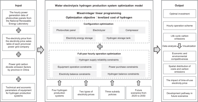
The optimization framework contains inputs, optimization models, and outputs. The optimization model is mixed-integer linear programming, the optimization objective is to minimize the levelized cost of hydrogen, and the decision variables include configuration and full-year hourly operation.

The optimization model for the water electrolysis hydrogen production system, such as WE3, is as follows. The code is available in the Supplementary Software. Optimization objectives, decision variables, and constraints are the three necessary parts for the optimization model. The optimization models for WE1, WE2, and WE4 are provided in Supplementary Note 1. The parameters and data involved in the optimization model are listed in Supplementary Note 2.

Water electrolysis hydrogen production optimization model

The LCOH is an internationally recognized economic evaluation indicator for the hydrogen energy industry. It represents the levelized monetary cost required to produce 1 kg of hydrogen throughout full life cycle of a hydrogen production project. A lower LCOH indicates lower hydrogen production costs for this technology pathway, and higher market competitiveness⁵. The LCOH for WE3 can be calculated as follows:

where LCOH_WE3 is the LCOH of the water electrolysis hydrogen production system, C_inv,WE3, C_om,WE3, C_grid,WE3 and C_c,WE3 are respectively the cost of investment, the cost of operation and maintenance throughout full life cycle, the cost of power purchase throughout full life cycle, and the cost of carbon emissions throughout full life cycle of the system. r is discount rate, %. N is life, years. c_inv,PV, c_inv,EL, c_inv,EES, c_inv,HST, c_inv,com are the cost of unit investment of photovoltaic panels, electrolyzer, electricity energy storage, hydrogen storage tanks, and compressors respectively. c_om,PV, c_om,EL, c_om,EES, c_om,HST, c_om,com are the costs of unit operation and maintenance of photovoltaic panels, electrolyzer, electricity energy storage, hydrogen storage tanks, and compressors respectively. The technical and economic parameters of each equipment are shown in Supplementary Table 1. c_grid is the purchase price of electricity, $/kW. c_grid,fix1 and c_grid,fix2 are the maximum demand price and transformer capacity price respectively, $/kW-year and $/kVA-year, φ is the phase angle. The retail electricity price of 35 kV large-scale industrial electricity is used as the representative electricity price for purchasing electricity from the grid. The electricity prices in each province are shown in Supplementary Table 2. c_c is the cost of carbon emission, $/t; LCCE_WE3 is the LCCE of the WE3.

Decision variables include system configuration and operation. The decision variables of configuration include the capacity of photovoltaic panels (IC_PV, kW), the capacity of electrolyzer (IC_EL, kW), the capacity of compressor (IC_com, kW), and the capacity of electricity energy storage (IC_EES, kWh), the capacity of the hydrogen storage tank (IC_HST, kg). The decision variables of operation include the input power of the electrolyzer (EP_EL(t), kW), the production of hydrogen of the electrolyzer (H_EL(t), kg), the power consumption of the compressor (EP_com(t), kW), the charging power of the electricity energy storage (EP_EES,im(t), kW), the discharging power of the electricity energy storage (EP_EES,ex(t), kW), hydrogen storage of the hydrogen storage tank (H _HST,im(t), kg), hydrogen release of the hydrogen storage tank (H _HST,ex(t), kg), power purchased from the grid (EP_grid(t), kW).

Equipment operation constraints

The annual photovoltaic power generation data of each province in the country is shown in Supplementary Fig. 1. Photovoltaic power generation and photovoltaic capacity are required to meet the following constraints^42,43.

where EP_PV is electric power output of photovoltaic panels, kW. EP_PV,0 is the output electric power of the photovoltaic panel with a rated capacity of 1 kW. IC_PV is the installation capacity of photovoltaic panels, kW.

The electrolyzer generates hydrogen by consuming electricity to electrolyze water. The energy conversion model is shown in Eq. (8). The input power and capacity of the electrolyzer are required to meet the constraints of Eqs. (9) and (10) respectively²⁷.

where EP_EL is the input electric power, kW. H_EL is the production of hydrogen, kg; IC_EL is the installation capacity of electrolyzer, kW. η_EL is the conversion efficiency of the electrolyzer, LHV is the lower calorific value of hydrogen, 33.3 kWh/kg.

The compressor compresses hydrogen to 200 bar and stores it in hydrogen storage tank. When hydrogen storage is needed, the compressor starts. This process is required to meet the following constraints³³.

where EP_com,0 is the electrical energy required to compress 1 kg of hydrogen, kWh. EP_com is the hourly electrical energy consumption of the compressor, kW. IC_com is the capacity of the compressor, kW.

The lithium battery can be installed to store electricity to ensure a stable power supply for the electrolysis process, as shown in the mathematical model below⁴⁴.

where E_EES(t) is the electricity, kWh; SOC_EES(t) is the real-time state of charge; E_EES(t + 1) is the electricity after charging or discharging, kWh; α is the self-discharge rate; EP_EES,im and EP_EES,ex are charging power and discharging power, respectively, kW; η_EES,im and η_EES,ex are charging efficiency and discharging efficiency, respectively; EP_EES,im,max and EP_EES,ex,max are the maximum charging power and discharging power, respectively; IC_EES is the installation capacity, kWh; SOC_EES,min and SOC_EES,max are the minimum and maximum state of charge respectively. Equation (18) limits the charging and discharging at the same time of the electrical energy storage. Equation (19) ensures that the initial and final state of the electrical energy storage is consistent.

Surplus renewable electricity can also be used to produce hydrogen directly, and the hydrogen produced by the electrolyzer can be compressed and stored in hydrogen storage tanks to ensure the hydrogen supply. The pressure of hydrogen storage tank is 200 bar. The mathematical model of the hydrogen storage tank is as follows⁴⁵.

where m_HST is the quality of hydrogen, kg. H _HST,im and H _HST,ex are the rates of hydrogen import and export by the hydrogen storage tank, respectively, kg/h. LOH_HST is the level of hydrogen. H _HST,im,max and H _HST,ex,max are the maximum rates of hydrogen import and export, respectively, kg; IC_HST is the installation capacity, kg; LOH_HST,min and LOH_HST,max are the minimum and maximum level of hydrogen; Eq. (26) limits hydrogen import and export at the same time; Eq. (27) ensures that the initial and final state of the hydrogen storage tank is consistent.

Power purchase constraints

The system is required to meet the following power purchase constraints to ensure that 50% renewable energy penetration.

where EP_grid is the purchase electricity, kW; EP_grid,max is the upper limit of purchase electricity, kW; h is total hours per year, 8760.

Electricity balance constraints

The electricity balance constraint of the system are as follows.

Hydrogen energy balance constraints

The hydrogen produced by the electrolyzer can be supplied directly to users or stored through hydrogen storage tank. Therefore, the hydrogen energy balance constraint is as follows.

where H_EL,out is the hydrogen energy provided by the electrolyzer to the hydrogen energy application scenario, kg.

Hydrogen supply reliability constraints

Hydrogen supply is required to meet hourly reliability²⁹.

where H_output is the annual supply of hydrogen of the system, 8760 kg.

Hydrogen production from coal optimization model

The LCOH of CG is calculated as follows²⁷.

where LCOH_CG is the LCOH of CG. c_inv,CG is the investment cost of CG, $/kW. IC_CG is the optimal capacity, kW. c_om,CG is the operation and maintenance cost of CG, $/kW; c_coal is the price of unit coal, 81.5 $/t. c_c is the emission price of unit carbon dioxide, 4.1 $/t. λ_CG is the CO₂ released by the CG per 1 kg of hydrogen produced. η_CG is the conversion efficiency of CG. Difference exists on investment cost, conversion efficiency and carbon emission coefficient between CG + CCUS and CG⁴⁶. The technical and economic parameters of the two systems are shown in Supplementary Table 3.

Hydrogen production from natural gas optimization model

The LCOH of SMR is calculated as follows.

where C_inv,SMR, C_om,SMR, C_gas,SMR, C_grid,SMR, and C_c,SMR are the investment cost, operation and maintenance cost, purchase cost of natural gas, power purchase cost and carbon emission cost of SMR, respectively. c_inv,SMR is the investment cost of the reformer, $/kW H₂. IC_SMR is the capacity of the reformer, kW H₂. c_om,SMR is the operation and maintenance cost of the reformer, $/kW H₂-year. G_gas is the natural gas required to produce 1 kg of hydrogen, kg. EP_grid is electricity consumed to produce 1 kg of hydrogen, kWh. LCCE_SMR is the LCCE of SMR, kg. H_SMR is the hourly production of hydrogen of SMR, kg. Difference exists on investment costs, operation and maintenance costs, power consumption, natural gas consumption and direct coefficients of carbon emission between SMR + CCUS and SMR. The technical and economic parameters of the two systems are shown in Supplementary Table 4. c_gas is the price of natural gas, $/m³. The price of natural gas in each province is shown in Supplementary Table 5⁴⁷.

Hydrogen production from industry by-products

The LCOH and LCCE of various hydrogen production technologies from industry by-product are shown in Supplementary Table 6.

Environmental assessment

The life cycle carbon emissions of grid electricity and photovoltaic panels are considered in the water electrolysis hydrogen production system. The LCCE of the system can be calculated as follows.

where λ_PV is carbon emission factor throughout full life cycle of photovoltaic panels, 0.04 kg CO₂/kWh. λ_grid is the grid carbon emission factor, the carbon emission factors of each province are shown in Supplementary Table 7. Grid carbon emissions are not included in the off-grid hydrogen production system.

The LCCE of SMR include direct carbon emissions, indirect carbon emissions generated by power purchase, carbon emissions associated with natural gas production and processing, and carbon emissions leaked during the natural gas production process²⁹. The calculation is as follows.

where CA_SMR is the direct carbon emissions of SMR, kg CO₂/kg H₂; λ_gas is the carbon emission factor associated with natural gas production and processing, 0.3 kg CO₂/kg CH₄. β is the fraction of the natural gas input that leaks during natural gas production and processing (kg CH₄ leaked/kg CH₄ input), 4%. δ is global warming potential of CH₄ relative to CO₂, the 20-year global warming potential of 85 kg CO₂/kg CH₄ is selected because of the urgency to decarbonize in the next few decades and the short-lived nature of natural gas in the atmosphere^29,48.

Subsidy policies

The subsidized policies of hydrogen production issued by various provinces in China are researched and divided into three categories. The first category is electricity price concession, such as the Policy Measures to Optimize Energy Structure and Promote Green and Low Carbon Development in Chengdu Municipality⁴⁹. The second category is investment matching incentives for carbon reduction, such as the Several Policies and Measures to Support the High-quality Development of Hydrogen Energy and Hydrogen Fuel Cell Vehicles issued by Shenyang⁵⁰. The third category is production subsidies, such as the Relevant Support Policies of Karamay Municipality to Support the Development of Hydrogen Energy Industry⁵¹. Accordingly, three subsidy policies scenarios are set in this research.

Reporting summary

Further information on research design is available in the Nature Portfolio Reporting Summary linked to this article.